11. Advanced Scheduling Techniques

11.1 Use of Advanced Scheduling Techniques

Construction project scheduling is a topic that has received extensive research over a number of decades. The previous chapter described the fundamental scheduling techniques widely used and supported by numerous commercial scheduling systems. A variety of special techniques have also been developed to address specific circumstances or problems. With the availability of more powerful computers and software, the use of advanced scheduling techniques is becoming easier and of greater relevance to practice. In this chapter, we survey some of the techniques that can be employed in this regard. These techniques address some important practical problems, such as:

• scheduling in the face of uncertain estimates on activity durations,
• integrated planning of scheduling and resource allocation,
• scheduling in unstructured or poorly formulated circumstances.

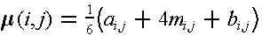
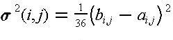
A final section in the chapter describes some possible improvements in the project scheduling process. In Chapter 14, we consider issues of computer based implementation of scheduling procedures, particularly in the context of integrating scheduling with other project management procedures.

11.2 Scheduling with Uncertain Durations

Section 10.3 described the application of critical path scheduling for the situation in which activity durations are fixed and known. Unfortunately, activity durations are estimates of the actual time required, and there is liable to be a significant amount of uncertainty associated with the actual durations. During the preliminary planning stages for a project, the uncertainty in activity durations is particularly large since the scope and obstacles to the project are still undefined. Activities that are outside of the control of the owner are likely to be more uncertain. For example, the time required to gain regulatory approval for projects may vary tremendously. Other external events such as adverse weather, trench collapses, or labor strikes make duration estimates particularly uncertain.

Two simple approaches to dealing with the uncertainty in activity durations warrant some discussion before introducing more formal scheduling procedures to deal with uncertainty. First, the uncertainty in activity durations may simply be ignored and scheduling done using the expected or most likely time duration for each activity. Since only one duration estimate needs to be made for each activity, this approach reduces the required work in setting up the original schedule. Formal methods of introducing uncertainty into the scheduling process require more work and assumptions. While this simple approach might be defended, it has two drawbacks. First, the use of expected activity durations typically results in overly optimistic schedules for completion; a numerical example of this optimism appears below. Second, the use of single activity durations often produces a rigid, inflexible mindset on the part of schedulers. As field managers appreciate, activity durations vary considerable and can be influenced by good leadership and close attention. As a result, field managers may loose confidence in the realism of a schedule based upon fixed activity durations. Clearly, the use of fixed activity durations in setting up a schedule makes a continual process of monitoring and updating the schedule in light of actual experience imperative. Otherwise, the project schedule is rapidly outdated.

A second simple approach to incorporation uncertainty also deserves mention. Many managers recognize that the use of expected durations may result in overly optimistic schedules, so they include a contingency allowance in their estimate of activity durations. For example, an activity with an expected duration of two days might be scheduled for a period of 2.2 days, including a ten percent contingency. Systematic application of this contingency would result in a ten percent increase in the expected time to complete the project. While the use of this rule-of-thumb or heuristic contingency factor can result in more accurate schedules, it is likely that formal scheduling methods that incorporate uncertainty more formally are useful as a means of obtaining greater accuracy or in understanding the effects of activity delays.

The most common formal approach to incorporate uncertainty in the scheduling process is to apply the critical path scheduling process (as described in Section 10.3) and then analyze the results from a probabilistic perspective. This process is usually referred to as the PERT scheduling or evaluation method. [1] As noted earlier, the duration of the critical path represents the minimum time required to complete the project. Using expected activity durations and critical path scheduling, a critical path of activities can be identified. This critical path is then used to analyze the duration of the project incorporating the uncertainty of the activity durations along the critical path. The expected project duration is equal to the sum of the expected durations of the activities along the critical path. Assuming that activity durations are independent random variables, the variance or variation in the duration of this critical path is calculated as the sum of the variances along the critical path. With the mean and variance of the identified critical path known, the distribution of activity durations can also be computed.

The mean and variance for each activity duration are typically computed from estimates of "optimistic" (a_i,j), "most likely" (m_i,j), and "pessimistic" (b_i,j) activity durations using the formulas:

(11.1)

and

(10.2)

where and are the mean duration and its variance, respectively, of an activity (i,j). Three activity durations estimates (i.e., optimistic, most likely, and pessimistic durations) are required in the calculation. The use of these optimistic, most likely, and pessimistic estimates stems from the fact that these are thought to be easier for managers to estimate subjectively. The formulas for calculating the mean and variance are derived by assuming that the activity durations follow a probabilistic beta distribution under a restrictive condition. [2] The probability density function of a beta distributions for a random varable x is given by:

(11.3)

;

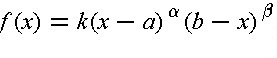
where k is a constant which can be expressed in terms of and . Several beta distributions for different sets of values of and are shown in Figure 11-1. For a beta distribution in the interval having a modal value m, the mean is given by:

(11.4)

If + = 4, then Eq. (11.4) will result in Eq. (11.1). Thus, the use of Eqs. (11.1) and (11.2) impose an additional condition on the beta distribution. In particular, the restriction that  = (b - a)/6 is imposed.

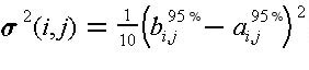
Figure 11-1  Illustration of Several Beta Distributions

Since absolute limits on the optimistic and pessimistic activity durations are extremely difficult to estimate from historical data, a common practice is to use the ninety-fifth percentile of activity durations for these points. Thus, the optimistic time would be such that there is only a one in twenty (five percent) chance that the actual duration would be less than the estimated optimistic time. Similarly, the pessimistic time is chosen so that there is only a five percent chance of exceeding this duration. Thus, there is a ninety percent chance of having the actual duration of an activity fall between the optimistic and pessimistic duration time estimates. With the use of ninety-fifth percentile values for the optimistic and pessimistic activity duration, the calculation of the expected duration according to Eq. (11.1) is unchanged but the formula for calculating the activity variance becomes:

(11.5)

The difference between Eqs. (11.2) and (11.5) comes only in the value of the divisor, with 36 used for absolute limits and 10 used for ninety-five percentile limits. This difference might be expected since the difference between b_i,j and a_i,j would be larger for absolute limits than for the ninety-fifth percentile limits.

While the PERT method has been made widely available, it suffers from three major problems. First, the procedure focuses upon a single critical path, when many paths might become critical due to random fluctuations. For example, suppose that the critical path with longest expected time happened to be completed early. Unfortunately, this does not necessarily mean that the project is completed early since another path or sequence of activities might take longer. Similarly, a longer than expected duration for an activity not on the critical path might result in that activity suddenly becoming critical. As a result of the focus on only a single path, the PERT method typically underestimates the actual project duration.

As a second problem with the PERT procedure, it is incorrect to assume that most construction activity durations are independent random variables. In practice, durations are correlated with one another. For example, if problems are encountered in the delivery of concrete for a project, this problem is likely to influence the expected duration of numerous activities involving concrete pours on a project. Positive correlations of this type between activity durations imply that the PERT method underestimates the variance of the critical path and thereby produces over-optimistic expectations of the probability of meeting a particular project completion deadline.

Finally, the PERT method requires three duration estimates for each activity rather than the single estimate developed for critical path scheduling. Thus, the difficulty and labor of estimating activity characteristics is multiplied threefold.

As an alternative to the PERT procedure, a straightforward method of obtaining information about the distribution of project completion times (as well as other schedule information) is through the use of Monte Carlo simulation. This technique calculates sets of artificial (but realistic) activity duration times and then applies a deterministic scheduling procedure to each set of durations. Numerous calculations are required in this process since simulated activity durations must be calculated and the scheduling procedure applied many times. For realistic project networks, 40 to 1,000 separate sets of activity durations might be used in a single scheduling simulation. The calculations associated with Monte Carlo simulation are described in the following section.

A number of different indicators of the project schedule can be estimated from the results of a Monte Carlo simulation:

• Estimates of the expected time and variance of the project completion.
• An estimate of the distribution of completion times, so that the probability of meeting a particular completion date can be estimated.
• The probability that a particular activity will lie on the critical path. This is of interest since the longest or critical path through the network may change as activity durations change.

The disadvantage of Monte Carlo simulation results from the additional information about activity durations that is required and the computational effort involved in numerous scheduling applications for each set of simulated durations. For each activity, the distribution of possible durations as well as the parameters of this distribution must be specified. For example, durations might be assumed or estimated to be uniformly distributed between a lower and upper value. In addition, correlations between activity durations should be specified. For example, if two activities involve assembling forms in different locations and at different times for a project, then the time required for each activity is likely to be closely related. If the forms pose some problems, then assembling them on both occasions might take longer than expected. This is an example of a positive correlation in activity times. In application, such correlations are commonly ignored, leading to errors in results. As a final problem and discouragement, easy to use software systems for Monte Carlo simulation of project schedules are not generally available. This is particularly the case when correlations between activity durations are desired.

Another approach to the simulation of different activity durations is to develop specific scenarios of events and determine the effect on the overall project schedule. This is a type of "what-if" problem solving in which a manager simulates events that might occur and sees the result. For example, the effects of different weather patterns on activity durations could be estimated and the resulting schedules for the different weather patterns compared. One method of obtaining information about the range of possible schedules is to apply the scheduling procedure using all optimistic, all most likely, and then all pessimistic activity durations. The result is three project schedules representing a range of possible outcomes. This process of "what-if" analysis is similar to that undertaken during the process of construction planning or during analysis of project crashing.

Example 11-1: Scheduling activities with uncertain time durations.

Suppose that the nine activity example project shown in Table 10-2 and Figure 10-4 of Chapter 10 was thought to have very uncertain activity time durations. As a result, project scheduling considering this uncertainty is desired. All three methods (PERT, Monte Carlo simulation, and "What-if" simulation) will be applied.

Table 11-1 shows the estimated optimistic, most likely and pessimistic durations for the nine activities. From these estimates, the mean, variance and standard deviation are calculated. In this calculation, ninety-fifth percentile estimates of optimistic and pessimistic duration times are assumed, so that Equation (11.5) is applied. The critical path for this project ignoring uncertainty in activity durations consists of activities A, C, F and I as found in Table 10-3 (Section 10.3). Applying the PERT analysis procedure suggests that the duration of the project would be approximately normally distributed. The sum of the means for the critical activities is 4.0 + 8.0 + 12.0 + 6.0 = 30.0 days, and the sum of the variances is 0.4 + 1.6 + 1.6 + 1.6 = 5.2 leading to a standard deviation of 2.3 days.

With a normally distributed project duration, the probability of meeting a project deadline is equal to the probability that the standard normal distribution is less than or equal to (PD - _D)|_D where PD is the project deadline, _D is the expected duration and _D is the standard deviation of project duration. For example, the probability of project completion within 35 days is:

where z is the standard normal distribution tabulated value of the cumulative standard distribution appears in Table B.1 of Appendix B.

Monte Carlo simulation results provide slightly different estimates of the project duration characteristics. Assuming that activity durations are independent and approximately normally distributed random variables with the mean and variances shown in Table 11-1, a simulation can be performed by obtaining simulated duration realization for each of the nine activities and applying critical path scheduling to the resulting network. Applying this procedure 500 times, the average project duration is found to be 30.9 days with a standard deviation of 2.5 days. The PERT result is less than this estimate by 0.9 days or three percent. Also, the critical path considered in the PERT procedure (consisting of activities A, C, F and I) is found to be the critical path in the simulated networks less than half the time.

TABLE 11-1  Activity Duration Estimates for a Nine Activity Project

Activity	Optimistic Duration	Most Likely Duration	Pessimistic Duration	Mean	Variance
A B C D E F G H I	3 2 6 5 6 10 2 4 4	4 3 8 7 9 12 2 5 6	5 5 10 8 14 14 4 8 8	4.0 3.2 8.0 6.8 9.3 12.0 2.3 5.3 6.0	0.4 0.9 1.6 0.9 6.4 1.6 0.4 1.6 1.6

If there are correlations among the activity durations, then significantly different results can be obtained. For example, suppose that activities C, E, G and H are all positively correlated random variables with a correlation of 0.5 for each pair of variables. Applying Monte Carlo simulation using 500 activity network simulations results in an average project duration of 36.5 days and a standard deviation of 4.9 days. This estimated average duration is 6.5 days or 20 percent longer than the PERT estimate or the estimate obtained ignoring uncertainty in durations. If correlations like this exist, these methods can seriously underestimate the actual project duration.

Finally, the project durations obtained by assuming all optimistic and all pessimistic activity durations are 23 and 41 days respectively. Other "what-if" simulations might be conducted for cases in which peculiar soil characteristics might make excavation difficult; these soil peculiarities might be responsible for the correlations of excavation activity durations described above.

Results from the different methods are summarized in Table 11-2. Note that positive correlations among some activity durations results in relatively large increases in the expected project duration and variability.

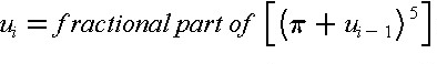
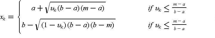
11.3 Calculations for Monte Carlo Schedule Simulation

In this section, we outline the procedures required to perform Monte Carlo simulation for the purpose of schedule analysis. These procedures presume that the various steps involved in forming a network plan and estimating the characteristics of the probability distributions for the various activities have been completed. Given a plan and the activity duration distributions, the heart of the Monte Carlo simulation procedure is the derivation of a realization or synthetic outcome of the relevant activity durations. Once these realizations are generated, standard scheduling techniques can be applied. We shall present the formulas associated with the generation of normally distributed activity durations, and then comment on the requirements for other distributions in an example.

To generate normally distributed realizations of activity durations, we can use a two step procedure. First, we generate uniformly distributed random variables, u_i in the interval from zero to one. Numerous techniques can be used for this purpose. For example, a general formula for random number generation can be of the form:

(11.6)

where = 3.14159265 and u_i-1 was the previously generated random number or a pre-selected beginning or seed number. For example, a seed of u₀ = 0.215 in Eq. (11.6) results in u₁ = 0.0820, and by applying this value of u₁, the result is u₂ = 0.1029. This formula is a special case of the mixed congruential method of random number generation. 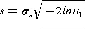While Equation (11.6) will result in a series of numbers that have the appearance and the necessary statistical properties of true random numbers, we should note that these are actually "pseudo" random numbers since the sequence of numbers will repeat given a long enough time.

With a method of generating uniformly distributed random numbers, we can generate normally distributed random numbers using two uniformly distributed realizations with the equations: [3]

(11.7)

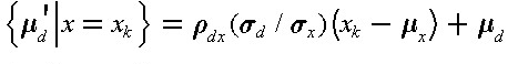
where x_k is the normal realization, _x is the mean of x, _x is the standard deviation of x, and u₁ and u₂ are the two uniformly distributed random variable realizations. For the case in which the mean of an activity is 2.5 days and the standard deviation of the duration is 1.5 days, a corresponding realization of the duration is s = 2.2365, t = 0.6465 and x_k = 2.525 days, using the two uniform random numbers generated from a seed of 0.215 above.

Correlated random number realizations may be generated making use of conditional distributions. For example, suppose that the duration of an activity d is normally distributed and correlated with a second normally distributed random variable x which may be another activity duration or a separate factor such as a weather effect. 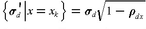Given a realization x_k of x, the conditional distribution of d is still normal, but it is a function of the value x_k. In particular, the conditional mean ('_d|x = x_k) and standard deviation ('_d|x = x_k) of a normally distributed variable given a realization of the second variable is:

(11.8)

where _dx is the correlation coefficient between d and x. Once x_k is known, the conditional mean and standard deviation can be calculated from Eq. (11.8) and then a realization of d obtained by applying Equation (11.7).

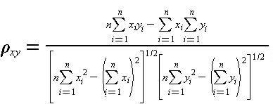
Correlation coefficients indicate the extent to which two random variables will tend to vary together. Positive correlation coefficients indicate one random variable will tend to exceed its mean when the other random variable does the same. From a set of n historical observations of two random variables, x and y, the correlation coefficient can be estimated as:

(11.9)

The value of _xy can range from one to minus one, with values near one indicating a positive, near linear relationship between the two random variables.

It is also possible to develop formulas for the conditional distribution of a random variable correlated with numerous other variables; this is termed a multi-variate distribution. [4] Random number generations from other types of distributions are also possible. [5] Once a set of random variable distributions is obtained, then the process of applying a scheduling algorithm is required as described in previous sections.

Example 11-2: A Three-Activity Project Example

Suppose that we wish to apply a Monte Carlo simulation procedure to a simple project involving three activities in series. As a result, the critical path for the project includes all three activities. We assume that the durations of the activities are normally distributed with the following parameters:

Activity	Mean (Days)	Standard Deviation (Days)
A B C	2.5 5.6 2.4	1.5 2.4 2.0

To simulate the schedule effects, we generate the duration realizations shown in Table 11-3 and calculate the project duration for each set of three activity duration realizations.

For the twelve sets of realizations shown in the table, the mean and standard deviation of the project duration can be estimated to be 10.49 days and 4.06 days respectively. In this simple case, we can also obtain an analytic solution for this duration, since it is only the sum of three independent normally distributed variables. The actual project duration has a mean of 10.5 days, and a standard deviation of days. With only a limited number of simulations, the mean obtained from simulations is close to the actual mean, while the estimated standard deviation from the simulation differs significantly from the actual value. This latter difference can be attributed to the nature of the set of realizations used in the simulations; using a larger number of simulated durations would result in a more accurate estimate of the standard deviation.

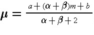
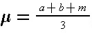
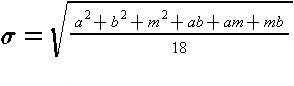
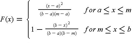
Example 11-3: Generation of Realizations from Triangular Distributions

To simplify calculations for Monte Carlo simulation of schedules, the use of a triangular distribution is advantageous compared to the normal or the beta distributions. Triangular distributions also have the advantage relative to the normal distribution that negative durations cannot be estimated. As illustrated in Figure 11-2, the triangular distribution can be skewed to the right or left and has finite limits like the beta distribution. If a is the lower limit, b the upper limit and m the most likely value, then the mean and standard deviation of a triangular distribution are:

(11.10)

(11.11)

The cumulative probability function for the triangular distribution is:

(11.12)

where F(x) is the probability that the random variable is less than or equal to the value of x.

Figure 11-2  Illustration of Two Triangular Activity Duration Distributions

Generating a random variable from this distribution can be accomplished with a single uniform random variable realization using the inversion method. In this method, a realization of the cumulative probability function, F(x) is generated and the corresponding value of x is calculated. Since the cumulative probability function varies from zero to one, the density function realization can be obtained from the uniform value random number generator, Equation (11.6). The calculation of the corresponding value of x is obtained from inverting Equation (11.12):

(11.13)

For example, if a = 3.2, m = 4.5 and b = 6.0, then _x = 4.8 and _x = 2.7. With a uniform realization of u = 0.215, then for (m-a)/(b-a) 0.215, x will lie between a and m and is found to have a value of 4.1 from Equation (11.13).

11.4 Crashing and Time/Cost Tradeoffs

The previous sections discussed the duration of activities as either fixed or random numbers with known characteristics. However, activity durations can often vary depending upon the type and amount of resources that are applied. Assigning more workers to a particular activity will normally result in a shorter duration. [6] Greater speed may result in higher costs and lower quality, however. In this section, we shall consider the impacts of time, cost and quality tradeoffs in activity durations. In this process, we shall discuss the procedure of project crashing as described below.

A simple representation of the possible relationship between the duration of an activity and its direct costs appears in Figure 11-3. Considering only this activity in isolation and without reference to the project completion deadline, a manager would undoubtedly choose a duration which implies minimum direct cost, represented by D_ij and C_ij in the figure. Unfortunately, if each activity was scheduled for the duration that resulted in the minimum direct cost in this way, the time to complete the entire project might be too long and substantial penalties associated with the late project start-up might be incurred. This is a small example of sub-optimization, in which a small component of a project is optimized or improved to the detriment of the entire project performance. Avoiding this problem of sub-optimization is a fundamental concern of project managers.

Figure 11-3  Illustration of a Linear Time/Cost Tradeoff for an Activity

At the other extreme, a manager might choose to complete the activity in the minimum possible time, D^c_ij, but at a higher cost C^c_ij. This minimum completion time is commonly called the activity crash time. The linear relationship shown in the figure between these two points implies that any intermediate duration could also be chosen. It is possible that some intermediate point may represent the ideal or optimal trade-off between time and cost for this activity.

What is the reason for an increase in direct cost as the activity duration is reduced? A simple case arises in the use of overtime work. By scheduling weekend or evening work, the completion time for an activity as measured in calendar days will be reduced. However, premium wages must be paid for such overtime work, so the cost will increase. Also, overtime work is more prone to accidents and quality problems that must be corrected, so indirect costs may also increase. More generally, we might not expect a linear relationship between duration and direct cost, but some convex function such as the nonlinear curve or the step function shown in Figure 11-4. A linear function may be a good approximation to the actual curve, however, and results in considerable analytical simplicity. [7]

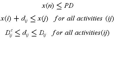
Figure 11-4  Illustration of Non-linear Time/Cost Tradeoffs for an Activity

With a linear relationship between cost and duration, the critical path time/cost tradeoff problem can be defined as a linear programming optimization problem. In particular, let R_ij represent the rate of change of cost as duration is decreased, illustrated by the absolute value of the slope of the line in Figure 11-3. Then, the direct cost of completing an activity is:

(11.14)

where the lower case c_ij and d_ij represent the scheduled duration and resulting cost of the activity ij. The actual duration of an activity must fall between the minimum cost time (D_ij) and the crash time (D^c_ij). Also, precedence constraints must be imposed as described earlier for each activity. Finally, the required completion time for the project or, alternatively, the costs associated with different completion times must be defined. Thus, the entire scheduling problem is to minimize total cost (equal to the sum of the c_ij values for all activities) subject to constraints arising from (1) the desired project duration, PD, (2) the minimum and maximum activity duration possibilities, and (3) constraints associated with the precedence or completion times of activities. Algebraically, this is:

(11.15)

where the notation is defined above and the decision variables are the activity durations d_ij and event times x(k). The appropriate schedules for different project durations can be found by repeatedly solving this problem for different project durations PD. The entire problem can be solved by linear programming or more efficient algorithms which take advantage of the special network form of the problem constraints.

One solution to the time-cost tradeoff problem is of particular interest and deserves mention here. The minimum time to complete a project is called the project-crash time. This minimum completion time can be found by applying critical path scheduling with all activity durations set to their minimum values (D^c_ij). This minimum completion time for the project can then be used in the time-cost scheduling problem described above to determine the minimum project-crash cost. Note that the project crash cost is not found by setting each activity to its crash duration and summing up the resulting costs; this solution is called the all-crash cost. Since there are some activities not on the critical path that can be assigned longer duration without delaying the project, it is advantageous to change the all-crash schedule and thereby reduce costs.

Heuristic approaches are also possible to the time/cost tradeoff problem. In particular, a simple approach is to first apply critical path scheduling with all activity durations assumed to be at minimum cost (D_ij). Next, the planner can examine activities on the critical path and reduce the scheduled duration of activities which have the lowest resulting increase in costs. In essence, the planner develops a list of activities on the critical path ranked in accordance with the unit change in cost for a reduction in the activity duration. The heuristic solution proceeds by shortening activities in the order of their lowest impact on costs. As the duration of activities on the shortest path are shortened, the project duration is also reduced. Eventually, another path becomes critical, and a new list of activities on the critical path must be prepared. By manual or automatic adjustments of this kind, good but not necessarily optimal schedules can be identified. Optimal or best schedules can only be assured by examining changes in combinations of activities as well as changes to single activities. However, by alternating between adjustments in particular activity durations (and their costs) and a critical path scheduling procedure, a planner can fairly rapidly devise a shorter schedule to meet a particular project deadline or, in the worst case, find that the deadline is impossible of accomplishment.

This type of heuristic approach to time-cost tradeoffs is essential when the time-cost tradeoffs for each activity are not known in advance or in the case of resource constraints on the project. In these cases, heuristic explorations may be useful to determine if greater effort should be spent on estimating time-cost tradeoffs or if additional resources should be retained for the project. In many cases, the basic time/cost tradeoff might not be a smooth curve as shown in Figure 11-4, but only a series of particular resource and schedule combinations which produce particular durations. For example, a planner might have the option of assigning either one or two crews to a particular activity; in this case, there are only two possible durations of interest.

Example 11-4: Time/Cost Trade-offs

The construction of a permanent transitway on an expressway median illustrates the possibilities for time/cost trade-offs in construction work. [8] One section of 10 miles of transitway was built in 1985 and 1986 to replace an existing contra-flow lane system (in which one lane in the expressway was reversed each day to provide additional capacity in the peak flow direction). Three engineers' estimates for work time were prepared:

• 975 calendar day, based on 750 working days at 5 days/week and 8 hours/day of work plus 30 days for bad weather, weekends and holidays.
• 702 calendar days, based on 540 working days at 6 days/week and 10 hours/day of work.
• 360 calendar days, based on 7 days/week and 24 hours/day of work.

The savings from early completion due to operating savings in the contra-flow lane and contract administration costs were estimated to be $5,000 per day.

In accepting bids for this construction work, the owner required both a dollar amount and a completion date. The bidder's completion date was required to fall between 360 and 540 days. In evaluating contract bids, a $5,000 credit was allowed for each day less than 540 days that a bidder specified for completion. In the end, the successful bidder completed the project in 270 days, receiving a bonus of 5,000*(540-270) = $450,000 in the $8,200,000 contract. However, the contractor experienced fifteen to thirty percent higher costs to maintain the continuous work schedule.

Example 11-5: Time cost trade-offs and project crashing

As an example of time/cost trade-offs and project crashing, suppose that we needed to reduce the project completion time for a seven activity product delivery project first analyzed in Section 10.3 as shown in Table 10-4 and Figure 10-7. Table 11-4 gives information pertaining to possible reductions in time which might be accomplished for the various activities. Using the minimum cost durations (as shown in column 2 of Table 11-4), the critical path includes activities C,E,F,G plus a dummy activity X. The project duration is 32 days in this case, and the project cost is $70,000.

TABLE 11-4  Activity Durations and Costs for a Seven Activity Project

Activity	Minimum Cost	Normal Duration	Crash Cost	Crash Duration	Change in Cost per Day
A B C D E F G	8 4 8 10 10 20 10	6 1 8 5 9 12 3	14 4 24 24 18 36 18	4 1 4 3 5 6 2	3 --- 4 7 2 2.7 8

Examining the unit change in cost, R_ij shown in column 6 of Table 11-4, the lowest rate of change occurs for activity E. Accordingly, a good heuristic strategy might be to begin by crashing this activity. The result is that the duration of activity E goes from 9 days to 5 days and the total project cost increases by $8,000. After making this change, the project duration drops to 28 days and two critical paths exist: (1) activities C,X,E,F and G, and (2) activities C, D, F, and G.

Examining the unit changes in cost again, activity F has the lowest value of R_ijj. Crashing this activity results in an additional time savings of 6 days in the project duration, an increase in project cost of $16,000, but no change in the critical paths. The activity on the critical path with the next lowest unit change in cost is activity C. Crashing this activity to its minimum completion time would reduce its duration by 4 days at a cost increase of $16,000. However, this reduction does not result in a reduction in the duration of the project by 4 days. After activity C is reduced to 7 days, then the alternate sequence of activities A and B lie on the critical path and further reductions in the duration of activity C alone do not result in project time savings. Accordingly, our heuristic corrections might be limited to reducing activity C by only 1 day, thereby increasing costs by $4,000 and reducing the project duration by 1 day.

At this point, our choices for reducing the project duration are fairly limited. We can either reduce the duration of activity G or, alternatively, reduce activity C and either activity A or activity B by an identical amount. Inspection of Table 11-4 and Figure 10-4 suggest that reducing activity A and activity C is the best alternative. Accordingly, we can shorten activity A to its crash duration (from 6 days to 4 days) and shorten the duration of activity C (from 7 days to 5 days) at an additional cost of $6,000 + $8,000 = $14,000. The result is a reduction in the project duration of 2 days.

Our last option for reducing the project duration is to crash activity G from 3 days to 2 days at an increase in cost of $8,000. No further reductions are possible in this time since each activity along a critical path (comprised of activities A, B, E, F and G) are at minimum durations. At this point, the project duration is 18 days and the project cost is $120,000., representing a fifty percent reduction in project duration and a seventy percent increase in cost. Note that not all the activities have been crashed. Activity C has been reduced in duration to 5 days (rather than its 4 day crash duration), while activity D has not been changed at all. If all activities had been crashed, the total project cost would have been $138,000, representing a useless expenditure of $18,000. The change in project cost with different project durations is shown graphically in Figure 11-5.

Figure 11-5  Project Cost Versus Time for a Seven Activity Project

Example 11-8: Mathematical Formulation of Time-Cost Trade-offs

The same results obtained in the previous example could be obtained using a formal optimization program and the data appearing in Tables 10-4 and 11-4. In this case, the heuristic approach used above has obtained the optimal solution at each stage. Using Eq. (11.15), the linear programming problem formulation would be:

Minimize   z
	= [8+3(6-dA)] + [4] + [8+4(8-dC)] + [10+7(5-dD)]
	+ [10+2(9-dE)] + [20+2.7(9-dF)] + [10+2(3-dG)]

subject to the constraints

x(6) = PD x(0) + d_A x(2)
x(0) + d_C x(1)
x(1) x(3)
x(2) + d_B x(4)
x(1) + d_D x(4)
x(2) + d_E x(4)
x(4) + d_F x(5)
x(5) + d_G x(6)
x(0) = 0
4 d_A 6
1 d_B 1
4 d_C 8
3 d_D 5
5 d_E 9
6 d_F 12
2 d_G 3

which can be solved for different values of project duration PD using a linear programming algorithm or a network flow algorithm. Note that even with only seven activities, the resulting linear programming problem is fairly large.

11.5 Scheduling in Poorly Structured Problems

The previous discussion of activity scheduling suggested that the general structure of the construction plan was known in advance. With previously defined activities, relationships among activities, and required resources, the scheduling problem could be represented as a mathematical optimization problem. Even in the case in which durations are uncertain, we assumed that the underlying probability distribution of durations is known and applied analytical techniques to investigate schedules.

While these various scheduling techniques have been exceedingly useful, they do not cover the range of scheduling problems encountered in practice. In particular, there are many cases in which costs and durations depend upon other activities due to congestion on the site. In contrast, the scheduling techniques discussed previously assume that durations of activities are generally independent of each other. A second problem stems from the complexity of construction technologies. In the course of resource allocations, numerous additional constraints or objectives may exist that are difficult to represent analytically. For example, different workers may have specialized in one type of activity or another. With greater experience, the work efficiency for particular crews may substantially increase. Unfortunately, representing such effects in the scheduling process can be very difficult. Another case of complexity occurs when activity durations and schedules are negotiated among the different parties in a project so there is no single overall planner.

A practical approach to these types of concerns is to insure that all schedules are reviewed and modified by experienced project managers before implementation. This manual review permits the incorporation of global constraints or consideration of peculiarities of workers and equipment. Indeed, interactive schedule revision to accomadate resource constraints is often superior to any computer based heuristic. With improved graphic representations and information availability, man-machine interaction is likely to improve as a scheduling procedure.

More generally, the solution procedures for scheduling in these more complicated situations cannot be reduced to mathematical algorithms. The best solution approach is likely to be a "generate-and-test" cycle for alternative plans and schedules. In this process, a possible schedule is hypothesized or generated. This schedule is tested for feasibility with respect to relevant constraints (such as available resources or time horizons) and desireability with respect to different objectives. Ideally, the process of evaluating an alternative will suggest directions for improvements or identify particular trouble spots. These results are then used in the generation of a new test alternative. This process continues until a satisfactory plan is obtained.

Two important problems must be borne in mind in applying a "generate-and-test" strategy. First, the number of possible plans and schedules is enormous, so considerable insight to the problem must be used in generating reasonable alternatives. Secondly, evaluating alternatives also may involve considerable effort and judgment. As a result, the number of actual cycles of alternative testing that can be accomadated is limited. One hope for computer technology in this regard is that the burdensome calculations associated with this type of planning may be assumed by the computer, thereby reducing the cost and required time for the planning effort. Some mechanisms along these lines are described in Chapter 15.

Example 11-9: Man-machine Interactive Scheduling

An interactive system for scheduling with resource constraints might have the following characteristics: [9]

• graphic displays of bar charts, resource use over time, activity networks and other graphic images available in different windows of a screen simultaneously,
• descriptions of particular activities including allocated resources and chosen technologies available in windows as desired by a user,
• a three dimensional animation of the construction process that can be stopped to show the progress of construction on the facility at any time,
• easy-to-use methods for changing start times and allocated resources, and
• utilities to run relevant scheduling algorithms such as the critical path method at any time.

Figure 11-6 shows an example of a screen for this system. In Figure 11-6, a bar chart appears in one window, a description of an activity in another window, and a graph of the use of a particular resource over time appears in a third window. These different "windows" appear as sections on a computer screen displaying different types of information. With these capabilities, a project manager can call up different pictures of the construction plan and make changes to accomadate objectives or constraints that are not formally represented. With rapid response to such changes, the effects can be immediately evaluated.

Figure 11-6  Example of a Bar Chart and Other Windows for Interactive Scheduling

11.6 Improving the Scheduling Process

Despite considerable attention by researchers and practitioners, the process of construction planning and scheduling still presents problems and opportunities for improvement. The importance of scheduling in insuring the effective coordination of work and the attainment of project deadlines is indisputable. For large projects with many parties involved, the use of formal schedules is indispensable.

The network model for representing project activities has been provided as an important conceptual and computational framework for planning and scheduling. Networks not only communicate the basic precedence relationships between activities, they also form the basis for most scheduling computations.

As a practical matter, most project scheduling is performed with the critical path scheduling method, supplemented by heuristic procedures used in project crash analysis or resource constrained scheduling. Many commercial software programs are available to perform these tasks. Probabilistic scheduling or the use of optimization software to perform time/cost trade-offs is rather more infrequently applied, but there are software programs available to perform these tasks if desired.

Rather than concentrating upon more elaborate solution algorithms, the most important innovations in construction scheduling are likely to appear in the areas of data storage, ease of use, data representation, communication and diagnostic or interpretation aids. Integration of scheduling information with accounting and design information through the means of database systems is one beneficial innovation; many scheduling systems do not provide such integration of information. The techniques discussed in Chapter 14 are particularly useful in this regard.

With regard to ease of use, the introduction of interactive scheduling systems, graphical output devices and automated data acquisition should produce a very different environment than has existed. In the past, scheduling was performed as a batch operation with output contained in lengthy tables of numbers. Updating of work progress and revising activity duration was a time consuming manual task. It is no surprise that managers viewed scheduling as extremely burdensome in this environment. The lower costs associated with computer systems as well as improved software make "user friendly" environments a real possibility for field operations on large projects.

Finally, information representation is an area which can result in substantial improvements. While the network model of project activities is an extremely useful device to represent a project, many aspects of project plans and activity inter-relationships cannot or have not been represented in network models. For example, the similarity of processes among different activities is usually unrecorded in the formal project representation. As a result, updating a project network in response to new information about a process such as concrete pours can be tedious. What is needed is a much more flexible and complete representation of project information. Some avenues for change along these lines are discussed in Chapter 15.

11.7 References

1. Bratley, Paul, Bennett L. Fox and Linus E. Schrage, A Guide to Simulation, Springer-Verlag, 1973.
2. Elmaghraby, S.E., Activity Networks: Project Planning and Control by Network Models, John Wiley, New York, 1977.
3. Jackson, M.J., Computers in Construction Planning and Control, Allen & Unwin, London, 1986.
4. Moder, J., C. Phillips and E. Davis, Project Management with CPM, PERT and Precedence Diagramming, Third Edition, Van Nostrand Reinhold Company, 1983.

11.8 Problems

1. For the project defined in Problem 1 from Chapter 10, suppose that the early, most likely and late time schedules are desired. Assume that the activity durations are approximately normally distributed with means as given in Table 10-16 and the following standard deviations: A: 4; B: 10; C: 1; D: 15; E: 6; F: 12; G: 9; H: 2; I: 4; J: 5; K: 1; L: 12; M: 2; N: 1; O: 5. (a) Find the early, most likely and late time schedules, and (b) estimate the probability that the project requires 25% more time than the expected duration.
   
   
2. For the project defined in Problem 2 from Chapter 10, suppose that the early, most likely and late time schedules are desired. Assume that the activity durations are approximately normally distributed with means as given in Table 10-17 and the following standard deviations: A: 2, B: 2, C: 1, D: 0, E: 0, F: 2; G: 0, H: 0, I: 0, J: 3; K: 0, L: 3; M: 2; N: 1. (a) Find the early, most likely and late time schedules, and (b) estimate the probability that the project requires 25% more time than the expected duration.

3 to 6

The time-cost tradeoff data corresponding to each of the Problems 1 to 4 (in Chapter 10), respectively are given in the table for the problem (Tables 11-5 to 11-8). Determine the all-crash and the project crash durations and cost based on the early time schedule for the project. Also, suggest a combination of activity durations which will lead to a project completion time equal to three days longer than the project crash time but would result in the (approximately) maximum savings.

TABLE 11-5 

Activity	A	B	C	D	E	F	G	H	I	J	K	L	M	N	O
Shortest Possible Completion Time	3	5	1	10	4	6	6	2	4	3	3	3	2	2	5
Normal Completion Time Cost	150	250	80	400	220	300	260	120	200	180	220	500	100	120	500
Change in Cost Per Day Earlier Completion	20	30	Infinity	15	20	25	10	35	20	Infinity	25	15	30	Infinity	10

TABLE 11-6 

Activity	A	B	C	D	E	F	G	H	I	J	K	L	M	N
Shortest Possible Completion Time	2	4	1	3	3	5	2	1	2	6	1	4	3	2
Normal Completion Time Cost	400	450	200	300	350	550	250	180	150	480	120	500	280	220
Crash Completion Time Cost	460	510	250	350	430	640	300	250	150	520	150	560	320	260

TABLE 11-7 

Activity	A	B	C	D	E	F	G	H	I	J	K	L
Shortest Possible Completion Time	4	8	11	4	1	9	6	2	3	2	7	3
Normal Completion Time Cost	70	150	200	60	40	120	100	50	70	60	120	70
Crash Completion Time Cost	90	210	250	80	60	140	130	70	90	80	150	100

TABLE 11-8 

Activity	A	B	C	D	E	F	G	H	I	J	K	L	M
Shortest Possible Completion Time	3	5	2	2	5	3	5	6	6	4	5	2	2
Normal Completion Time Cost	50	150	90	125	300	240	80	270	120	600	300	80	140
Change in Cost Per Day Earlier Completion	Infinity	50	Infinity	40	30	20	15	30	Infinity	40	50	40	40

7 to 10

Develop a project completion time versus cost tradeoff curve for the projects in Problems 3 to 6. (Note: a linear programming computer program or more specialized programs can reduce the calculating work involved in these problems!)

11. Suppose that the project described in Problem 5 from Chapter 10 proceeds normally on an earliest time schedule with all activities scheduled for their normal completion time. However, suppose that activity G requires 20 days rather than the expected 5. What might a project manager do to insure completion of the project by the originally planned completion time?
    
    
12. For the project defined in Problem 1 from Chapter 10, suppose that a Monte Carlo simulation with ten repetitions is desired. Suppose further that the activity durations have a triangular distribution with the following lower and upper bounds: A:4,8; B:4,9, C: 0.5,2; D: 10,20; E: 4,7; F: 7,10; G: 8, 12; H: 2,4; I: 4,7; J: 2,4; K: 2,6; L: 10, 15; M: 2,9; N: 1,4; O: 4,11.
    (a) Calculate the value of m for each activity given the upper and lower bounds and the expected duration shown in Table 10-16.
    (b) Generate a set of realizations for each activity and calculate the resulting project duration.
    (c) Repeat part (b) five times and estimate the mean and standard deviation of the project duration.
    
    
13. Suppose that two variables both have triangular distributions and are correlated. The resulting multi-variable probability density function has a triangular shape. Develop the formula for the conditional distribution of one variable given the corresponding realization of the other variable.

11.9 Footnotes

1. See D. G. Malcolm, J.H. Rosenbloom, C.E. Clark, and W. Fazar, "Applications of a Technique for R and D Program Evaluation," Operations Research, Vol. 7, No. 5, 1959, pp. 646-669. Back

2. See M.W. Sasieni, "A Note on PERT Times," Management Science, Vol. 32, No. 12, p 1986, p. 1652-1653, and T.K. Littlefield and P.H. Randolph, "An Answer to Sasieni's Question on Pert Times," Management Science, Vol. 33, No. 10, 1987, pp. 1357-1359. For a general discussion of the Beta distribution, see N.L. Johnson and S. Kotz, Continuous Univariate Distributions-2, John Wiley & Sons, 1970, Chapter 24. Back

3. See T. Au, R.M. Shane, and L.A. Hoel, Fundamentals of Systems Engineering - Probabilistic Models, Addison-Wesley Publishing Company, 1972. Back

4. See N.L. Johnson and S. Kotz, Distributions in Statistics: Continuous Multivariate Distributions, John Wiley & Sons, New York, 1973. Back

5. See, for example, P. Bratley, B. L. Fox and L.E. Schrage, A Guide to Simulation, Springer-Verlag, New York, 1983. Back

6. There are exceptions to this rule, though. More workers may also mean additional training burdens and more problems of communication and management. Some activities cannot be easily broken into tasks for numerous individuals; some aspects of computer programming provide notable examples. Indeed, software programming can be so perverse that examples exist of additional workers resulting in slower project completion. See F.P. Brooks, jr. , The Mythical Man-Month, Addison Wesley, Reading, MA 1975. Back

7. For a discussion of solution procedures and analogies of the general function time/cost tradeoff problem, see C. Hendrickson and B.N. Janson, "A Common Network Flow Formulation for Several Civil Engineering Problems," Civil Engineering Systems, Vol. 1, No. 4, 1984, pp. 195-203. Back

8. This example was abstracted from work performed in Houston and reported in U. Officer, "Using Accelerated Contracts with Incentive Provisions for Transitway Construction in Houston," Paper Presented at the January 1986 Transportation Research Board Annual Conference, Washington, D.C. Back

9. This description is based on an interactive scheduling system developed at Carnegie Mellon University and described in C. Hendrickson, C. Zozaya-Gorostiza, D. Rehak, E. Baracco-Miller and P. Lim, "An Expert System for Construction Planning," ASCE Journal of Computing, Vol. 1, No. 4, 1987, pp. 253-269. Back